Computational
Morphogenesis
A high-resolution atlas of pattern formation in Turing's reaction-diffusion space
In 1952, Alan Turing published his final paper — The Chemical Basis of Morphogenesis — proposing that the patterns on animal coats, seashells, and fish scales emerge from the interplay of two chemicals diffusing at different rates. He called this reaction-diffusion, and he worked out the mathematics on paper, years before computers could simulate it.
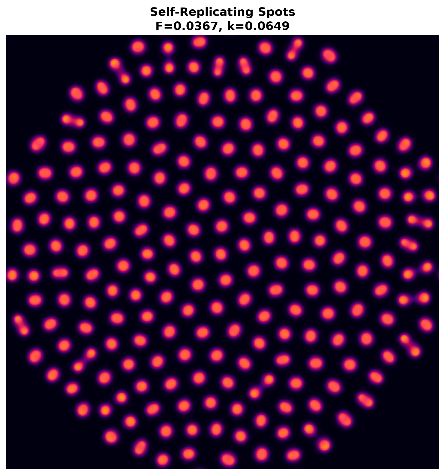
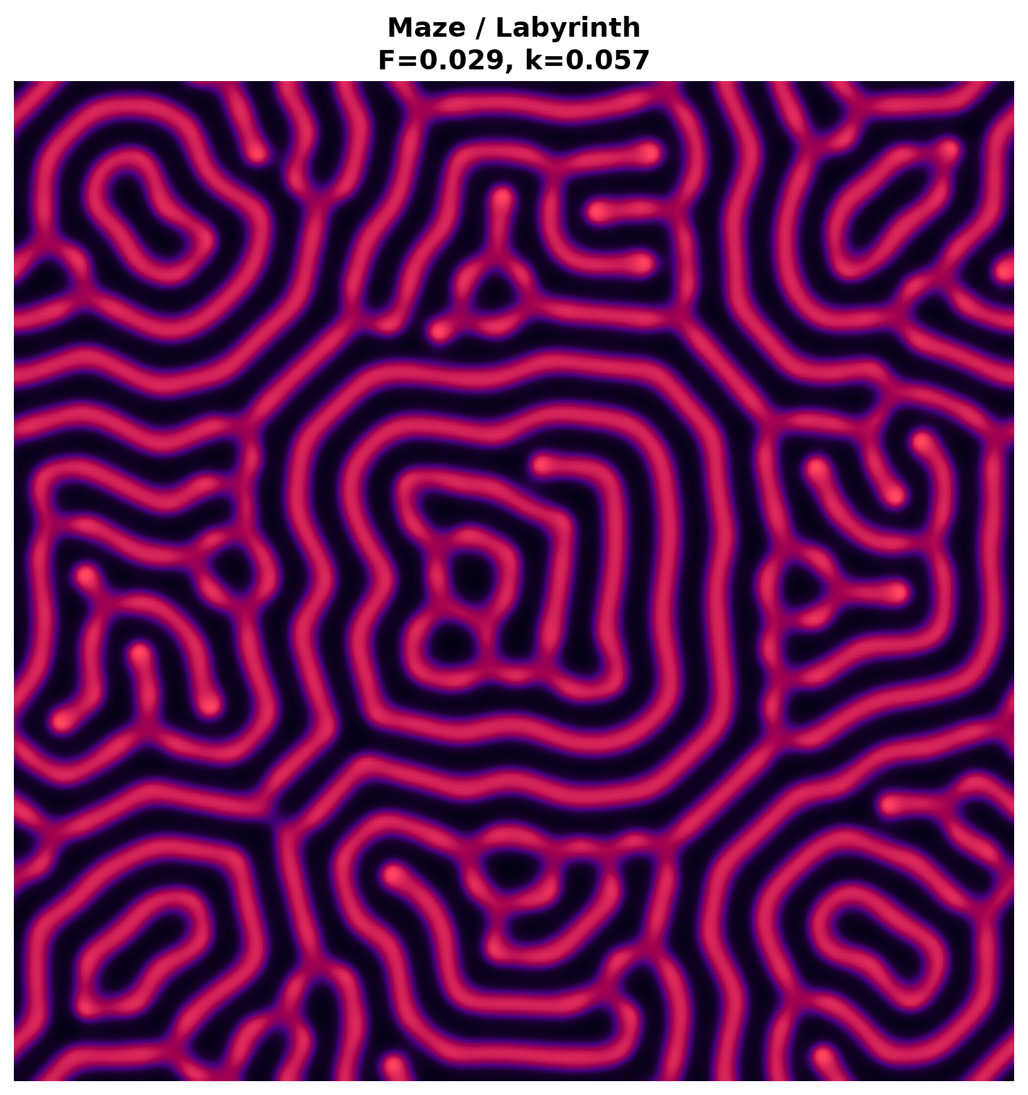
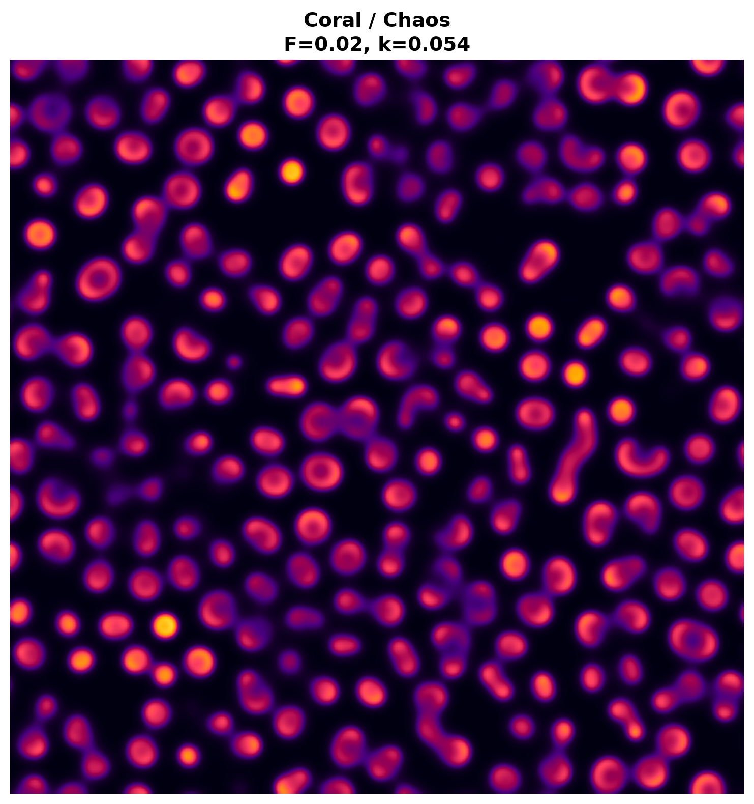
In 1993, John Pearson ran the Gray-Scott equations on a 1990s supercomputer and discovered a zoo of patterns no one had predicted: self-replicating spots, growing labyrinths, coral-like chaos, and oscillating worms. His Science paper revealed a system where simple rules produce stunning complexity.
Two chemicals. Two parameters. Infinite beauty.
This project re-creates and extends that exploration using modern hardware: a systematic sweep of 2,304 parameter combinations, each simulated from first principles in NumPy, then analyzed with linear stability theory to test what theory predicts and what actually happens.
- 01Gray-Scott is NOT a classical Turing system The trivial steady state (1, 0) is linearly stable everywhere — its Jacobian is diagonal. Patterns cannot arise from linear instability of the uniform state. They are finite-amplitude, nonlinear phenomena.
- 02Linear theory fails to predict wavelengths Where nontrivial steady states exist and are Turing-unstable, the predicted critical wavelength λ_c shows essentially no correlation with measured wavelengths (Pearson r = −0.244, n = 180).
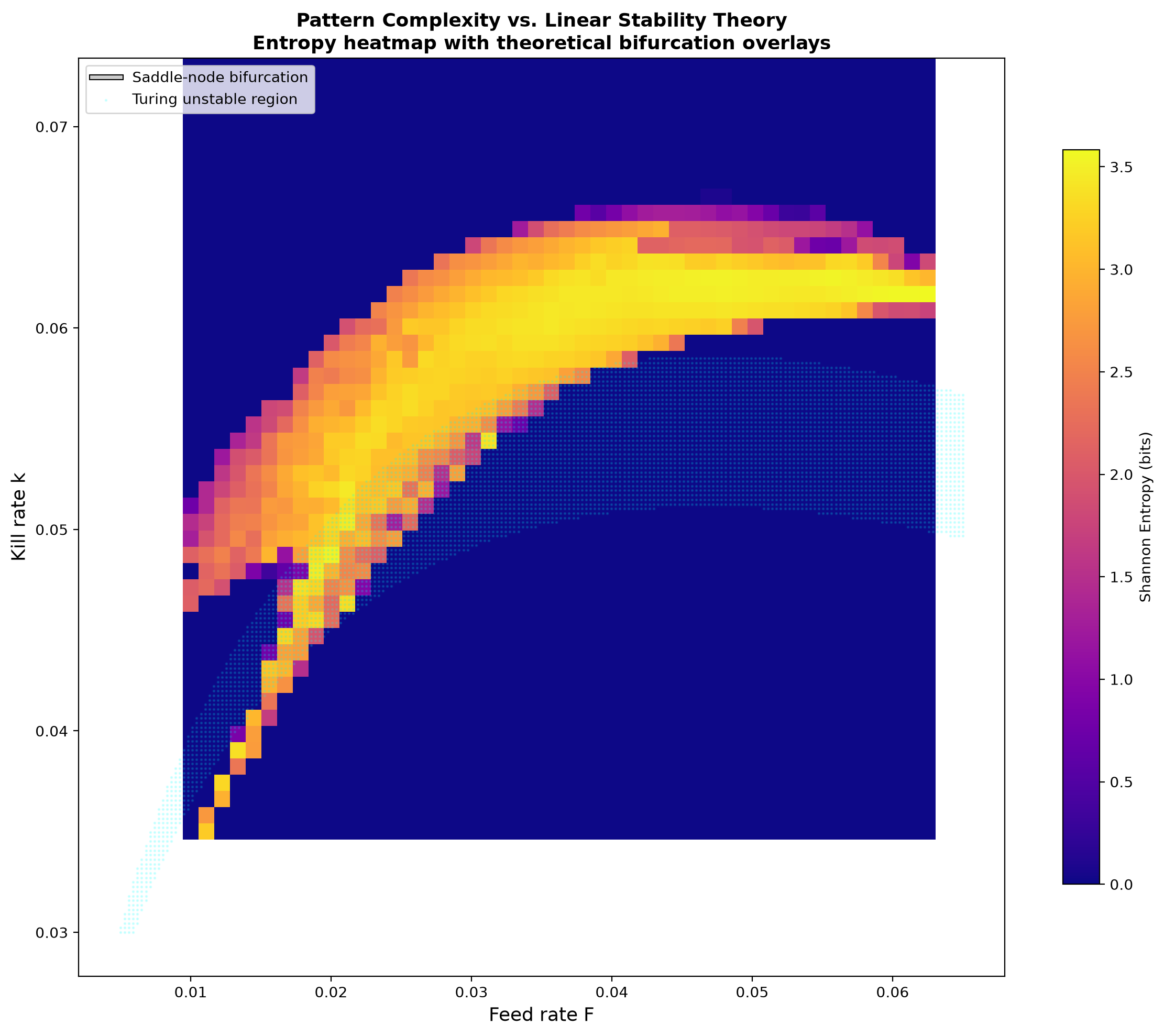
- 03The saddle-node boundary organizes everything The analytic bifurcation curve k_c = √F/4 − F precisely bounds the pattern-forming region. Inside the curve: complex patterns. Outside: death or saturation. The transition is pixel-sharp.
- 04Complexity peaks far from the boundary Shannon entropy of the pattern field increases with distance from the saddle-node bifurcation, contradicting the "critical slowing down" expectation. The richest patterns live deep in the pattern region, not at its edge.
Below: Shannon entropy of the concentration field across the full (F, k) parameter space. Bright regions are maximally complex patterns. Dark regions are uniform states. The white dashed curve is the analytically-derived saddle-node bifurcation — note how it precisely traces the phase boundary.
- Full Research Paper — complete methods, theory, results, and discussion
- Pattern Gallery — 9 showcase patterns at high resolution
- Raw Data & Code — CSV results, NumPy grids, reproducible Python
- More from Herman → — see this project on the main site, alongside other work